
Homework 2
Online Algorithm
An ‘online’ algorithm is one that is designed to handle processing input data that arrives in a sequence, and not as a complete set. Taking log events as a perfect example, this type of data arrives sequentially one event after the other. An ‘online’ algorithm is designed to process each new piece of data or log event as it arrives to produce a final result. Also note that such algorithms are not designed with any assumptions about future data that may arrive, such as how many events or when. These are the unknowns the algorithm designer must take into account.
The opposite would be an ‘offline’ (or ‘batch’) algorithm where the complete data set of interest is provided to the algorithm at the same time. Therefore the ‘offline’ algorithm will start out and finish with a known fixed number of data points.
As also explained in one measurement of the cost incurred by an ‘on-line’ algorithm is it’s ‘competitive ratio’, being the “maximum, over all possible input sequences, of the ratio between the cost incurred by the on-line algorithm and the cost incurred by an optimal off-line algorithm. An optimal on-line algorithm is then one whose competitive ratio is least”. Of course finding this ratio is easier said then done, and also note that not all ‘online’ algorithms have matching ‘offline’ equivalents.
B. P. Welford
With regard to the ‘online’ variance algorithm, this arose from the work of Scientist B. P. Welford who published a paper in 1962 on “a Method for Calculating Corrected Sums of Squares and Products” with an offered solution where values are used only once and need not be stored.
Standard Deviation
The Standard Deviation is a measurement of the dispersion of a set of data points. A low value indicates that the set of data points tend to be close to the mean (the expected value). In simple terms the Standard Deviation of a set of data points is the square root of variance.
Welford’s Algorithm
It is often useful to be able to compute the variance in a single pass, inspecting each value \(x_{i}\)only once; for example, when the data is being collected without enough storage to keep all the values, or when costs of memory access dominate those of computation. This is where the ‘online’ variance work done by B. P. Welford is relevant.
You can find Welford’s algorithm explained in Knuth’s 2nd volume Seminumerical Algorithms:
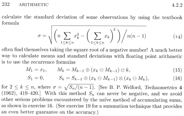 Those funny symbols ⊕⊖⊗⊘ are just there to designate the approximation operations of floating-point machine arithmetic, as opposed to the exact mathematical operators ”+”, “−”, “×”, “/”; when it comes to computations in floating-point, the computer is almost always inaccurate, even if the error is very small.
Rewritten in “normal” discrete-time math for clarity, our algorithm is this:
Those funny symbols ⊕⊖⊗⊘ are just there to designate the approximation operations of floating-point machine arithmetic, as opposed to the exact mathematical operators ”+”, “−”, “×”, “/”; when it comes to computations in floating-point, the computer is almost always inaccurate, even if the error is very small.
Rewritten in “normal” discrete-time math for clarity, our algorithm is this:
Update the Mean
Given the following stream: \(x[1], x[2], x[3], \dots, x[k]\) and the mean at the step k equals to: \(M[k] = \frac{1}{k} \sum_{i=1}^k x[i] = \frac{1}{k} \left( \sum_{i=1}^{k-1} x[i] + x[k] \right)\)
and \(\sum_{i=1}^{k-1} x[i] = (k-1) \ M[k-1]\)
compute: \(M[k] = \frac{1}{k} \left( (k-1) M[k-1] + x[k] \right)\)
\[M[k] = \frac {(k-1)}{k} M[k-1] + \frac {x[k]}{k}\] \[M[k] = 1⋅ M[k-1] - \frac {1}{k} M[k-1] + \frac {x[k]}{k}\] \[M[k] = M[k-1] + \frac{1}{k}\left(x[k] - M[k-1]\right)\]Update the Variance
\[\begin{eqnarray} k \cdot var[k] &=& \sum_{i=1}^{k} x^2[i] + x[k]^2 - k \cdot M^2[k],\\ &=& (k-1) \cdot var^2[k-1] + (k-1) \cdot M^2[k-1] + x^2[k] - k \cdot M[k]^2,\\ &=& (k-1) \cdot var^2[k-1] + (k-1) \cdot M^2[k-1] + x^2[k] - \frac{1}{k}(k-1) \cdot (M[k-1] + x^2[k])\\ &=& (k-1) \cdot var^2[k-1] + (k-1) \cdot M^2[k-1] + x^2[k] - \frac{1}{k}({(k-1)^2} M^2[k-1] + 2(k-1) \cdot M[k-1]x[k] + x^2[k]). \end{eqnarray}\] \[\begin{eqnarray} k^2 \cdot var^2[k] &=& (k-1) \cdot k \cdot var^2[k-1] + (k-1)(M^2[k-1] - 2M[k-1]x[k] + x^2[k]) \\ &=& (k-1) \cdot k \cdot var^2[k-1] + (k-1)(M[k-1] - x^2[k]). \end{eqnarray}\] \[\begin{eqnarray} var^2[k] &=& var^2[k-1] + \frac {(k-1)(M[k-1] - x^2[k]) - k \cdot var^2[k-1]} {k^2} \end{eqnarray}\] \[\begin{eqnarray} &~&\frac {(k-1)(M[k-1] - x[k])^2 - (k \cdot var^2[k-1]} {k^2} \\ &=& \frac {(x[k] - M[k-1])(k-1)(x[k] - M[k-1]) - (k \cdot var^2[k-1]} {k^2}\\ &=& \frac {(k-1)(x[k] - M[k-1])(k-1) \cdot k \cdot (M[k] - M[k-1]) - k \cdot var^2[k-1]} {k^2}\\ &=& \frac {(x[k] - M[k-1])(k-1)(M[k] - M[k-1]) - var^2[k-1]} {k} \\ &=& \frac {(x[k] - M[k-1])(x[k] - M[k] - var^2[k-1]} {k}.\\ \end{eqnarray}\] \[var[k] = var[k-1] + \frac { (x[k]-M[k-1])(x[k]-M[k]) - var[k-1]}{k}\]Here it is possible to isolate the value \(S\), which will be useful for calculating both the population variance and the sample variance.
\[S[k] = var[k] \cdot k = var[k-1] \cdot k + (x[k]-M[k-1])(x[k]-M[k]) - var[k-1]\] \[S[k] = var[k] \cdot k = (k-1) \cdot var[k-1] + (x[k]-M[k-1])(x[k]-M[k])\] \[S[k] = S[k-1] + \left(x[k]-M[k-1]\right)\left(x[k]-M[k]\right)\]Sample Variance: \(sampleVariance[k] = \frac {S[k]}{k - 1}\)
Population Variance: \(populationVariance[k] = \frac {S[k]}{k}\)
Algorithm Implementation
We can write Welford’s method in Python as follows:
'''
L'algoritmo aggiorna la media e S (che serve per calcolare la varianza) all'arrivo del valore x dallo stream
INPUT:
	x -> valore input (proveniente dallo stream)
	k -> contatore del numero di valori inviati dallo stream
	M -> media calcolata fino al passo k-1
	S -> valore che serve a calcolare la varianza, calcolato fino al passo k-1

	Nota: il calcolo della varianza viene svolto fuori dalla funzione di update
OUTPUT:
	Mnext -> Valore M aggiornato al passo k
	Snext -> Valore S aggiornato al passo k
'''
def welford_algorithm(x, k, M, S):
    if k == 1:
        return (x, 0)
    else:
        Mnext = M + (x - M) / k
        Snext = S + (x - M)*(x - Mnext)
        return (Mnext, Snext)

'''Funzione che simula il flusso di dati e stampa per ogni valore x la mediana, la varianza campionaria e la deviazione standard'''
def stream(data_stream):
    M = 0.0
    S = 0.0
    variance = 0.0
    k = 1
    for x in data_stream:
        # Aggiorna lo stato
        M, S = welford_algorithm(x, k, M, S)
        if k > 1:
            variance = S / (k - 1)  # Varianza campionaria
            stand_dev = math.sqrt(variance)
        print(f"x={x}, Mediana={M:.2f}, Varianza={variance:.2f}, \
        stand_dev={stand_dev:.2f}")
        k += 1

# Simuliamo il flusso di dati
data_stream = [2, 4, 4, 4, 5, 5, 7, 9]

# Eseguiamo l'algoritmo di Welford
stream(data_stream)
Accurancy
Like many statistical methods, it is more accurate if you can normalize the inputs, namely subtract off a gross estimate of the mean, and then scale by a gross estimate of standard deviation, leaving you with a normalized input x′ which has a mean closer to zero and a standard deviation closer to 1.0:
But for typical applications with 16-bit inputs, you can probably get away without bothering to normalize.
Practice
Personal Notes
Dynamics of Mean and Variance Over Time:
Relative Frequency in Bernoulli Processes:
As time progresses, the mean is expected to converge towards the probability \(p\). Although the variance may initially display significant fluctuations, it should stabilize as the number of trials increases, in accordance with the law of large numbers.
Absolute Frequency in Bernoulli Processes:
The mean typically exhibits a linear increase as the accumulation of successes occurs over time. Concurrently, the variance also escalates, as each success or failure contributes to the overall dispersion of the data.
Mean Behavior in Random Walks:
The mean trajectory in a random walk demonstrates an upward or downward trend, contingent upon the balance of positive and negative jumps (with a probability of \(p\)). The variance is observed to increase over time, indicating greater dispersion as the number of steps grows.
Relative Frequency in Random Walks:
The mean relative frequency tends to stabilize over time, akin to the behavior observed in the Bernoulli process, although it may exhibit more variability during the earlier stages. As the total number of steps increases, the variance generally decreases, ultimately converging around the probability \(p\).
Contrasting Absolute and Relative Frequency Distributions:
Characteristics of Relative Frequencies:
Conversely, the distribution of relative frequencies (proportions) converges towards the expected probability \(p\). Over time, the variance diminishes as the total number of observations increases, leading to enhanced stability and a narrower distribution around the mean.
Characteristics of Absolute Frequencies:
The distribution of absolute successes (for instance, in a Bernoulli process) tends to broaden over time, reflecting the cumulative nature of the process. This distribution becomes wider as variance increases with the number of steps, resulting in an expanded range of potential outcomes.
References
- Citation: Welford, B.P., 1962. Note on a method for calculating corrected sums of squares and products. Technometrics, 4(3), pp.419-420.
- Rapid7 Blog (2016). Overview of online algorithm using standard deviation example.
- Citation: Karp, R.M., 1992, August. On-line algorithms versus off-line algorithms: How much is it worth to know the future?. In IFIP Congress (1) (Vol. 12, pp. 416-429).